── Attaching core tidyverse packages ──────────────────────── tidyverse 2.0.0 ──
✔ dplyr     1.1.2     ✔ readr     2.1.4
✔ forcats   1.0.0     ✔ stringr   1.5.0
✔ ggplot2   3.4.2     ✔ tibble    3.2.1
✔ lubridate 1.9.2     ✔ tidyr     1.3.0
✔ purrr     1.0.1
── Conflicts ────────────────────────────────────────── tidyverse_conflicts() ──
✖ dplyr::filter() masks stats::filter()
✖ dplyr::lag()    masks stats::lag()
ℹ Use the conflicted package (<http://conflicted.r-lib.org/>) to force all conflicts to become errors

Attaching package: 'janitor'


The following objects are masked from 'package:stats':

    chisq.test, fisher.test


here() starts at /workspaces/report-elnino
Analysis: ways of measuring El Niño
For a few of these charts, we’re going to compare outcomes with an indicator measuring ENSO phase (El Niño, neutral or La Niña). But as ENSO is a phenomenon of both the atmosphere and the ocean, there’re a few ways to measure it. We’re going to compare those to see if it makes a lot of difference to our classifications.
On the ocean side, the NINO34 index—also called the Oceanic Nino Index (ONI)—defines sea surface temperatures in the mid-eastern Pacific. An anomaly in that area from the long term average of at least +0.5°C defines an El Niño, while lower than -0.5°C defines a La Niña.
On the atmospheric side, the Southern Oscillation Index (SOI) compares the air pressure difference between Tahiti and Darwin. An SOI below -8 for an extended period defines an El Niño; an SOI above +8 defines a La Niña.
ONI is NOAA’s primary index for El Ni˜no measurement, but the Australian Bureau of Meteorology typically looks at both (as well as dynamical factors and seasonal forecast models) to make the call.
Let’s load data in for both and compare. Nino3.4 comes from the NASA Physical Sciences Laboratory:
Warning: 17 parsing failures.
row  col               expected    actual                                                             file
155 year no trailing characters -99.99    '/workspaces/report-elnino/data/nasa-nino34-anomaly-monthly.txt'
155 NA   13 columns             1 columns '/workspaces/report-elnino/data/nasa-nino34-anomaly-monthly.txt'
156 year no trailing characters NINA34    '/workspaces/report-elnino/data/nasa-nino34-anomaly-monthly.txt'
156 NA   13 columns             1 columns '/workspaces/report-elnino/data/nasa-nino34-anomaly-monthly.txt'
157 year no trailing characters 5N-5S     '/workspaces/report-elnino/data/nasa-nino34-anomaly-monthly.txt'
... .... ...................... ......... ................................................................
See problems(...) for more details.
And here’s SOI over June-Sep each year:
Rows: 1769 Columns: 2
── Column specification ────────────────────────────────────────────────────────
Delimiter: ","
dbl (2): year_month, soi

ℹ Use `spec()` to retrieve the full column specification for this data.
ℹ Specify the column types or set `show_col_types = FALSE` to quiet this message.
Now we can join and compare the two:
When we demand that both indicators agree on a phase, we get a subset of the years manually indicated as an El Niño or La Niña by the Bureau of Meteorology. That could be because our indicators are focusing on June–September (partly because we’re interested in kharif crops later in this analysis), where some ENSO events might develop later (or maybe one of the ocean or atmosphere began later than the other).
If we go with at least one of the indicators in a phase (provided the two don’t disagree with opposite phases), we get a list more consistent with the BOM.
Analysis: Indian rainfall and ENSO
New names:
Rows: 609 Columns: 12
── Column specification
──────────────────────────────────────────────────────── Delimiter: "," chr
(1): ...1 dbl (11): Year, Actual Rainfall: JUN, Actual Rainfall: JUL, Actual
Rainfall:...
ℹ Use `spec()` to retrieve the full column specification for this data. ℹ
Specify the column types or set `show_col_types = FALSE` to quiet this message.
• `` -> `...1`
Analysis: monthly SOI to JJAS SOI
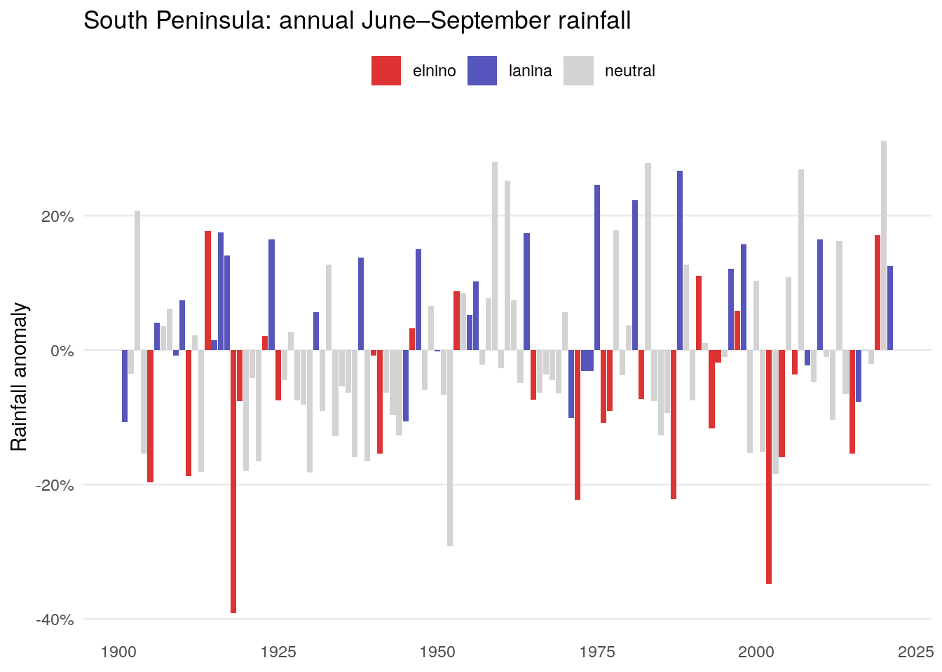
Let’s join the two and visualise by colour. Here’s the Southern Peninsula:
Analysis: crop yield and ENSO
Now let’s pull in crop yield data from ICRISAT. This data has columns for each crop and each of three measures:
- Area (in thousands of hectares),
- Productions (in thousands of tons), and
- Yield (in kilograms per hectare)
Let’s lengthen this a bit so that we can compute on all the dimensions, and we’ll classify the states according to the rainfall region that they’re in:
Rows: 16146 Columns: 80
── Column specification ────────────────────────────────────────────────────────
Delimiter: ","
chr  (2): State Name, Dist Name
dbl (78): Dist Code, Year, State Code, RICE AREA (1000 ha), RICE PRODUCTION ...

ℹ Use `spec()` to retrieve the full column specification for this data.
ℹ Specify the column types or set `show_col_types = FALSE` to quiet this message.
Production by region and crop
Now that this is tidy, let’s start wide.
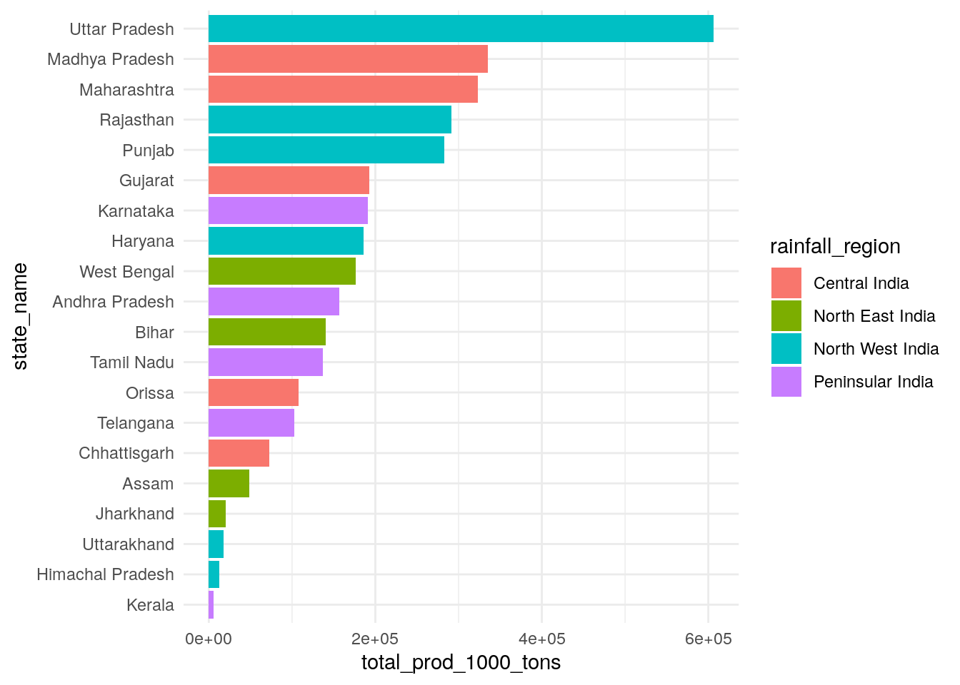
Before we start looking at breakdowns across regions and crops, let’s first just find out which regions and crops produce the most (in mass terms!)
`summarise()` has grouped output by 'state_name'. You can override using the
`.groups` argument.
Looks like biggest-producing states over 2005-2014 were all Central and North West region states.
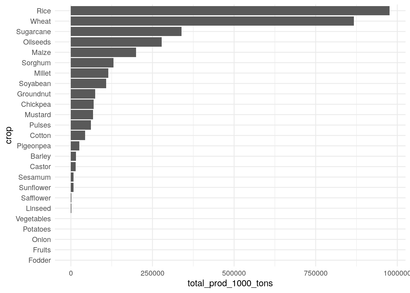
How about crops?
As expected, rice and wheat are big ones, followed by sugarcane, oilseeds and maize.
We probably want to focus on kharif crops, which are ones grown during the monsoon season that are dependent on good rain. Rice and maize are both major kharif crops, but wheat is not—it’s a rabi crop, grown in the winter.
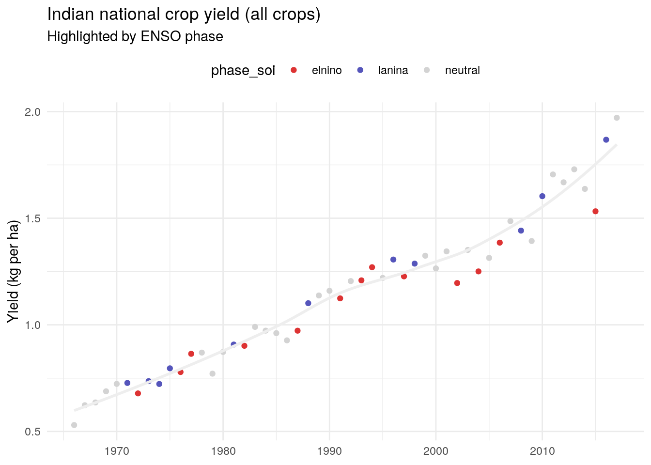
Annual yield (all regions and crops)
Note
Yield in kg/ha is (production * 10^6) / (area in * 10^3)
`geom_smooth()` using method = 'loess' and formula = 'y ~ x'
We can see that yield has increased steadily over time (likely thanks to technological improvements), but you can see a bit of year-to-year variation.
There’s a lot of noise here, as we’re looking at parts of India and crops that are less dependent on rainfall.
Yield by region
Let’s look at this two ways: all crops for each region, and each crop for all regions. We’ll start looking at each region:
`summarise()` has grouped output by 'year'. You can override using the
`.groups` argument.
`geom_smooth()` using method = 'loess' and formula = 'y ~ x'
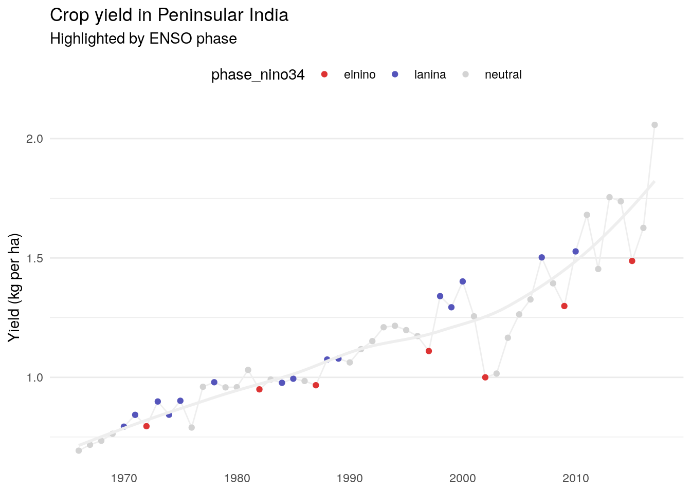
It’s interesting to see that yield variability has increased substantially in the last 20 years, particularly in Peninsular India.
`geom_smooth()` using method = 'loess' and formula = 'y ~ x'
# A tibble: 52 × 9
    year .fitted   .resid elnino_yield neutral_yield lanina_yield elnino_resid
   <dbl>   <dbl>    <dbl>        <dbl>         <dbl>        <dbl>        <dbl>
 1  1966   0.715 -0.0217        NA             0.693       NA           NA
 2  1967   0.733 -0.0155        NA             0.717       NA           NA
 3  1968   0.751 -0.0168        NA             0.734       NA           NA
 4  1969   0.769 -0.00525       NA             0.764       NA           NA
 5  1970   0.786  0.00689       NA            NA            0.793       NA
 6  1971   0.804  0.0392        NA            NA            0.843       NA
 7  1972   0.821 -0.0254         0.795        NA           NA            0.795
 8  1973   0.837  0.0616        NA            NA            0.899       NA
 9  1974   0.853 -0.00981       NA            NA            0.843       NA
10  1975   0.869  0.0328        NA            NA            0.902       NA
11  1976   0.885 -0.0950        NA             0.790       NA           NA
12  1977   0.900  0.0602        NA             0.960       NA           NA
13  1978   0.916  0.0637        NA            NA            0.979       NA
14  1979   0.931  0.0271        NA             0.958       NA           NA
15  1980   0.945  0.0137        NA             0.959       NA           NA
16  1981   0.958  0.0726        NA             1.03        NA           NA
17  1982   0.972 -0.0221         0.950        NA           NA            0.950
18  1983   0.985  0.00561       NA             0.991       NA           NA
19  1984   0.999 -0.0220        NA            NA            0.977       NA
20  1985   1.01  -0.0196        NA            NA            0.994       NA
21  1986   1.03  -0.0457        NA             0.985       NA           NA
22  1987   1.05  -0.0818         0.967        NA           NA            0.967
23  1988   1.07   0.00675       NA            NA            1.07        NA
24  1989   1.09  -0.00816       NA            NA            1.08        NA
25  1990   1.10  -0.0419        NA             1.06        NA           NA
26  1991   1.12  -0.00144       NA             1.12        NA           NA
27  1992   1.13   0.0199        NA             1.15        NA           NA
28  1993   1.14   0.0678        NA             1.21        NA           NA
29  1994   1.15   0.0650        NA             1.22        NA           NA
30  1995   1.16   0.0382        NA             1.20        NA           NA
31  1996   1.17   0.00391       NA             1.17        NA           NA
32  1997   1.18  -0.0700         1.11         NA           NA            1.11
33  1998   1.19   0.146         NA            NA            1.34        NA
34  1999   1.21   0.0847        NA            NA            1.29        NA
35  2000   1.22   0.179         NA            NA            1.40        NA
36  2001   1.24   0.0181        NA             1.26        NA           NA
37  2002   1.25  -0.254          1.00         NA           NA            1.00
38  2003   1.27  -0.258         NA             1.02        NA           NA
39  2004   1.30  -0.132         NA             1.17        NA           NA
40  2005   1.32  -0.0607        NA             1.26        NA           NA
41  2006   1.35  -0.0266        NA             1.33        NA           NA
42  2007   1.38   0.119         NA            NA            1.50        NA
43  2008   1.42  -0.0214        NA             1.39        NA           NA
44  2009   1.45  -0.151          1.30         NA           NA            1.30
45  2010   1.49   0.0409        NA            NA            1.53        NA
46  2011   1.53   0.154         NA             1.68        NA           NA
47  2012   1.57  -0.116         NA             1.45        NA           NA
48  2013   1.62   0.139         NA             1.75        NA           NA
49  2014   1.66   0.0738        NA             1.74        NA           NA
50  2015   1.71  -0.226          1.49         NA           NA            1.49
51  2016   1.77  -0.141         NA             1.63        NA           NA
52  2017   1.82   0.235         NA             2.06        NA           NA
# ℹ 2 more variables: neutral_resid <dbl>, lanina_resid <dbl>

The strong relationship here in Peninsular India, with a weaker relationship in Central India.
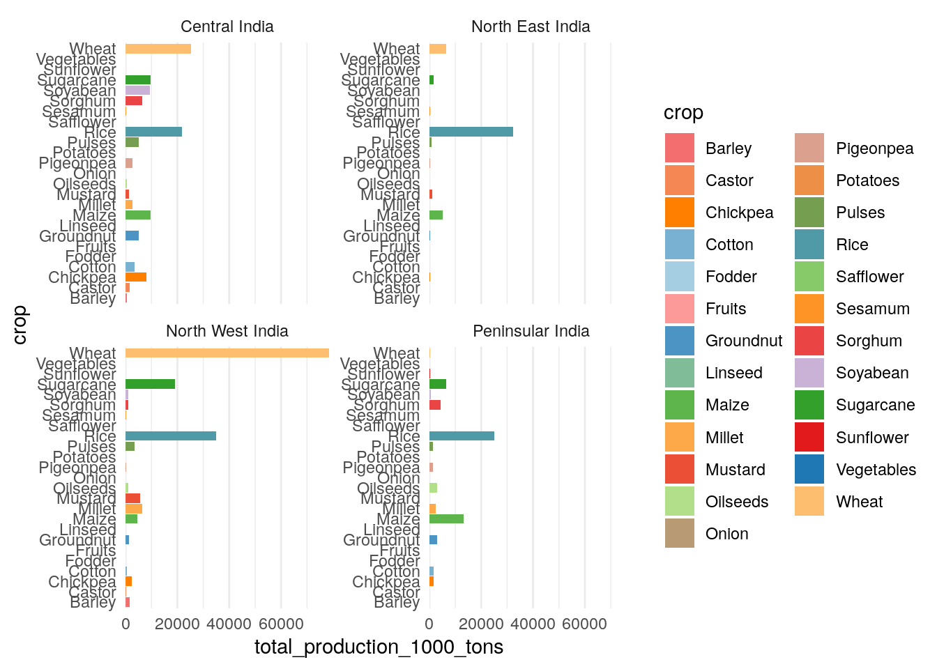
Crops grown by region
`summarise()` has grouped output by 'rainfall_region'. You can override using
the `.groups` argument.
Rice is a major crop in all four regions—Peninsular India contributed around 25 million tonnes in 2022 (about 20% of the national total).
Maize is another crop grown in this season, and Peninsular India is a major grower—about 13 million tonnes (about 40% of the national total).
The other big crops in
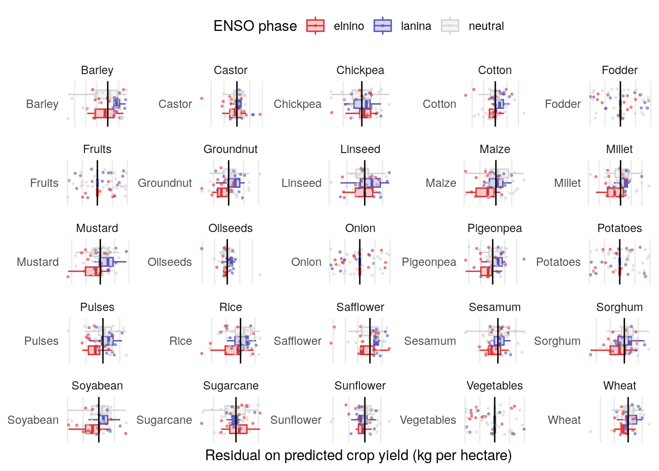
Yield by crop
`summarise()` has grouped output by 'year'. You can override using the
`.groups` argument.
Crops that seem to be most affected by ENSO include Groundnut, Cotton, Pigeonpea, Pulses and Soyabean. Others with a possible but marginal-looking relationship include Maize, Millet, Mustard, Oilseed, Safflower and Rice.
Analysis: crop yield and rainfall
That said, using SOI directly as a predictor might not be the way to go. It might be helpful to look at rainfall more directly as a predictor and then see the effect of ENSO on top.
The first thing we’ll need to do is match Indian states to rainfall regions (NE, NW, central, peninsular). Then we can join the rainfall and crop yield datasets.
`summarise()` has grouped output by 'year', 'rainfall_region'. You can override
using the `.groups` argument.
It still looks like the stronger relationship here is with certain crops rather than certain regions, but let’s break it down by both.
Analysis: ENSO and global and national temperatures
Here, global and national temperatures are courtesy of Berkeley Earth. They have generously agreed to licence the data here under Creative Commons Attribution (CC BY 4.0).
Let’s start with global temperature data:
Warning: 1 parsing failure.
row col   expected    actual                                                               file
  1  -- 12 columns 1 columns '/workspaces/report-elnino/data/berkeley-monthly-tavg-ecuador.txt'
Warning: 1 parsing failure.
row col   expected    actual                                                               file
  1  -- 12 columns 1 columns '/workspaces/report-elnino/data/berkeley-monthly-tavg-florida.txt'
Warning: 1 parsing failure.
row col   expected    actual                                                              file
  1  -- 12 columns 1 columns '/workspaces/report-elnino/data/berkeley-monthly-tavg-global.txt'
Warning: 1 parsing failure.
row col   expected    actual                                                                 file
  1  -- 12 columns 1 columns '/workspaces/report-elnino/data/berkeley-monthly-tavg-indonesia.txt'
Warning: 1 parsing failure.
row col   expected    actual                                                                file
  1  -- 12 columns 1 columns '/workspaces/report-elnino/data/berkeley-monthly-tavg-malaysia.txt'
Warning: 1 parsing failure.
row col   expected    actual                                                                   file
  1  -- 12 columns 1 columns '/workspaces/report-elnino/data/berkeley-monthly-tavg-new_zealand.txt'
Warning: 1 parsing failure.
row col   expected    actual                                                             file
  1  -- 12 columns 1 columns '/workspaces/report-elnino/data/berkeley-monthly-tavg-texas.txt'
Let’s join it to the Nino3.4, which we have monthly across the whole year. But we might need a smoother on those first.
Warning: There was 1 warning in `mutate()`.
ℹ In argument: `date = ymd(paste(year, month, "01"))`.
Caused by warning:
!  6 failed to parse.
First let’s look at the global picture:
Warning: Removed 24 rows containing missing values (`geom_segment()`).
Warning: Removed 24 rows containing missing values (`geom_line()`).
Warning: Removed 24 rows containing missing values (`geom_segment()`).
Warning: Removed 24 rows containing missing values (`geom_line()`).
And then some selected regions:
Warning: Removed 11 rows containing missing values (`geom_segment()`).
Warning: Removed 31 rows containing missing values (`geom_segment()`).
Warning: Removed 30 rows containing missing values (`geom_segment()`).
Warning: Removed 11 rows containing missing values (`geom_line()`).
Warning: Removed 11 rows containing missing values (`geom_segment()`).
Warning: Removed 31 rows containing missing values (`geom_segment()`).
Warning: Removed 30 rows containing missing values (`geom_segment()`).
Warning: Removed 11 rows containing missing values (`geom_line()`).